4 Adult Galaxias Maculatus Recruitment is Shaped by Juvenile Growth and Hatch Date

4.1 Introduction

An individual’s chance of surviving to successfully reproduce may be affected by a variety of factors. Fitness may be linked to size, condition, growth, and hatch date (Anderson 1988, Jakob et al. 1996, Jacob et al. 2009, Buston and Elith 2011) and therefore fish may experience selective mortality by any or all of these characteristics. Selection on phenotypes is widely recognised across ecosystems, but the mechanisms are often system- (Houde 1989, Kaemingk et al. 2013) and context-dependent (Cargnelli and Gross 1996, Garvey et al. 2002). Temporal variation in the biotic and abiotic factors of an environment can lead to selective pressures on larval fish that vary based on an individual’s hatch date (Cargnelli and Gross 1996). Both hatch date (Lande and Arnold 1983, Kohler et al. 1993, Cargnelli and Gross 1996, Santucci Jr and Wahl 2003) and growth history (Leggett and Deblois 1994, Sogard 1997) have been linked to survivorship in fish. Selective pressures may act on both these traits to preferentially favour fish that have hatched at the ‘right time’ (Garvey et al. 2002), grew at an optimum rate (Crecco and Savoy 1985), or some combination of these two factors. If larval fish show high phenotypic plasticity, which may offer increased survivorship (Burgess and Marshall 2011, Burgess et al. 2012), then the combination of phenotypic plasticity and hatching over a broad temporal time scale may offer a population the best chance of successful recruitment.

A substantial body of evidence indicates that hatching at the ‘right time’ can positively influence an individual’s developmental trajectory and future success. Early hatch dates may be beneficial due to increased developmental time (Divino and Tonn 2007), as older and larger fish often experience the highest survival to year one (Cargnelli and Gross 1996). Old and large fish may also be the first to spawn in a population, and also produce the largest eggs (Simpson 1959), which creates a feedback loop where the offspring of early spawners may be more likely to become early spawners in the next generation. Larger fish may also experience higher survivorship due to having excess fat reserves to exploit in periods of starvation (Bagenal 1971). However, while there may be ecological benefits to early hatching, potential benefits may simply be a function of hatching at the ‘right time.’ For example, variation in hatch date may lead to different cohorts of larvae experiencing different seasonal characteristics such as food availability or temperature differences (Cushing 1969, Kohler et al. 1993, Santucci Jr and Wahl 2003, Kaemingk et al. 2013). Specific hatch dates may increase fitness in early life stages, but subsequently decrease fitness in later stages (Langerhans et al. 2004, Bogner et al. 2016). This variation in fitness is often linked to hatch-dependent growth rate (Divino and Tonn 2007), where post-hatch experiences have subsequent effects on an individual’s growth rate. Earlier hatch dates are often linked with size-dependent mortality as fish born earlier have more time to grow and are less likely to perish (Divino and Tonn 2007). This ‘bigger-is-better’ hypothesis works under the assumption that a larger fish is either too big for a predator to consume (i.e., gape limited) and/or has the swimming ability to evade capture (Hovenkamp 1992, Meekan and Fortier 1996). However, there is also evidence of slower growth being beneficial, as this can lead to higher levels of predator avoidance (Amara et al. 1994, Gleason and Bengtson 1996). Selection can operate on growth rates (Shima and Findlay 2002), and therefore ultimately determine survivorship (Rosenberg and Haugen 1982). In species with high variation in demographic rates, early life history can be an indicator of rearing environment (Svanback and Eklov 2002). Fish that have developed in warm, productive environments are more likely to be larger, have a faster growth rate, and have more energy reserves to dedicate to reproduction (Houde 1989). Therefore, early life history can be used to predict future success if we know that a certain set of traits will be beneficial for an individual at a later life stage (Houde 1997). By sampling a population repeatedly through time it is possible to identify changes in the distribution of phenotypes (Vigliola et al. 2007). In species with recruitment that occurs over a period of time, the range of recruiting phenotypes may vary through time, and therefore the survivors among these cohorts would possess traits necessary for future success (Cargnelli and Gross 1996).

The aim of this chapter is to understand how both hatch date and growth rate of juvenile fish independently shape adult populations. To address this question I sampled discrete populations of pre-settlement juveniles throughout the peak recruitment season (McDowall et al. 1994). I sampled the populations again six months later (post-settlement), after those cohorts of fish had reached maturity. As fish will likely experience different sources of mortality post-settlement and pre-settlement, I hypothesized that mortality would be selective with respect to hatch date and/or growth rate. Therefore, I expect to see reduced variation in these traits when the surviving adults are sampled. Given that fish entering the rivers early in the recruitment season have faster average growth rates (see chapter 2) that may confer increased fitness, I hypothesized that early hatched recruits would have increased chances of survival. Therefore, I expected fish that entered the river in August to comprise the majority of the adult population.

4.2 Methods

4.2.1 Fish collections

I used otolith daily ring formations to characterize hatch dates and growth histories for two life stages of the amphidromous fish Galaxias maculatus. After hatching from eggs laid in riparian vegetation, larvae spend approximately 6 months developing in marine areas where they have opportunity to disperse (McDowall 1968). Fish will then migrate to, and settle in, freshwater streams where they will spend another six months developing into reproductively mature adults (McDowall 1968). I caught fish from each life stage at two rivers to test whether adult fish had similar growth histories and hatch dates to juvenile fish.

I sampled juveniles and adults from the Hutt River and the Wainuiomata River. Juveniles were sampled over a period of months, and details of this sampling are given in chapter 2. For analysis of growth rate I assigned sampled fish to specific ‘cohorts’ based upon their month of collection. Juvenile fish were not grouped into cohorts for analysis of hatch date.

I sampled these cohorts again approximately six months later, after the juveniles had developed into adult fish and were ready to spawn. My sampling regime makes the assumption that I am sampling the same set of cohorts in each life history stage without any bias. It also assumes that G. maculatus lives for one year and is semelparous (but see Stevens et al. 2016). While recent evidence suggests that some individuals survive through to year 2 and display iteroparity, the aging of all samples would detect any year 2 fish, and therefore would not skew the results. I sampled adult G. maculatus from spawning grounds (i.e. riparian vegetation covering moist riverbanks, Benzie 1968a) and used two unbaited sock nets to catch adult fish. I only fished on days where the high tide was ≥ 1.8 metres. The nets were set 2-3 hours before the high tide, and were taken down approximately one hour after high tide. The total sample size was 50 adult fish. Twenty fish were caught from the Wainuiomata River on 19th March 2016. Thirty fish were caught from the Hutt River over 8 separate fishing days, spread from 25th March to 5 June 2016.

4.2.2 Otolith analyses

Adult otoliths were prepared identically to the juvenile otolith preparation described in chapter 2. Briefly, age was estimated as the number of daily rings visible between the core and the edge of the otolith along the postrostral axis. The complete otolith growth history was characterised by measuring the distance between each successive ring along the postrostral axis. I used the age of each fish to back-calculate hatch dates of individuals. For analysis, I converted hatch dates to a numerical ‘day of the year’ (Julian date).

4.2.3 Statistical analysis

I hypothesised that the sample of adult fish would show a different hatch distribution to that of the juvenile fish sample due to selective mortality. I also hypothesised that the sample of adult fish would show a similar growth history to one or more of the monthly cohorts of juveniles sampled, likely favouring faster growth. I tested each site separately for the null hypothesis that both adult and juvenile fish hatch dates were drawn from a common population using an Anderson-Darling test and a one-way ANOVA test. The Anderson-Darling test compares the shape of the hatch date distributions (Scholz and Stephens 1987) while the ANOVA compares the mean value of the distributions, under the assumption of a normal distribution. Significant differences in these tests would therefore suggest the adult population hatched at a different time to the juveniles. The Anderson-Darling test does not have its own unique distribution (unlike the chi-squared test). Therefore, although a test statistic and an approximate p-value can be calculated, there is no way to calculate critical values or degrees of freedom (Anderson and Darling 1954). Results of the Anderson-Darling test and the ANOVA result are presented as density plots to account for the large difference in sample sizes between adults and juveniles.

I used a linear mixed-effects model to test whether cohorts of juvenile fish had different otolith growth curves to the adult fish cohort. I truncated all otolith growth data to a maximum of 180 days (the average juvenile age) to avoid any effect of post-settlement otolith growth from the adult fish. I modelled individual growth trajectories for each fish (juveniles and adults) by using size-at-age of the otolith as the response variable. Therefore, each fish had n repeated measures where n is equal to the age of the fish, up to a maximum of 180 days. I included a random slope and intercept for ‘Fish ID’ to (1) allow for the relationship between age and otolith growth to vary across individuals and (2) allow for correlation in daily rings within each individual. I used ‘age’ (in days) as the continuous variable to predict the size of the otolith. The model also included a cohort variable that accounted for four monthly juvenile groups (August, September, October, November) and one adult group of fish (5 levels total). The cohort variable was included as a fixed effect to test differences in growth histories between the adult fish and each monthly cohort of juvenile fish. I was not interested in comparing any of the juvenile cohort’s otolith growth histories to each other: each juvenile cohort was only compared to the adult otolith growth history, as my hypothesis was based around which juvenile cohort(s) was similar to the adult population. This model calculated an overall slope for each level of cohort (based on the relationship between otolith size and age), which I interpreted as an estimate of otolith growth rate for each cohort. I used Wald t scores to compare the otolith growth estimate of each juvenile cohort to the otolith growth estimate of the adult cohort. Each site was modelled separately to facilitate these comparisons, and to account for potential site-specific patterns (see Chapter 2). All mixed models were run using ‘lme’ from the ‘nlme’ package (Pinheiro et al. 2016) in RStudio v0.99.903 (RStudio Team 2015).

From the mixed model I obtained estimates of the otolith growth rate for each juvenile cohort. Wald t tests were calculated in the mixed model by setting one level of the categorical factor (the cohort variable) as a reference level. Adult fish were set as the reference level, and so all estimates of juvenile growth are calculated relative to the adult fish. Therefore any juvenile cohorts that had an equal growth rate to the adult cohort would have an estimate equal to zero.

4.3 Results

4.3.1 Shifts in juvenile hatch dates

Results of the Anderson-Darling test suggest that the distributions of hatch dates for adult and juvenile fish in the Hutt River did not come from a common distribution (T = 26.09, p < 0.0001). On average, juveniles had a hatchdate 47 days earlier than adult fish (F1, 339 = 49.602, p < 0.0001, 4.1). Adult and juvenile fish in the Wainuiomata River had hatchdates that were drawn from a common distribution (T = 0.1761, p = 0.2937). Adult and juvenile fish had hatchdates approximately 7 days apart, but this difference was not significant (F1, 201 = 0.88, p = 0.3493). A density plot represents the probability density function of a continuous random variable (in this case, day of the year). Therefore, it allows for easy visualisation of the two distribution curves, despite the difference in sample sizes.

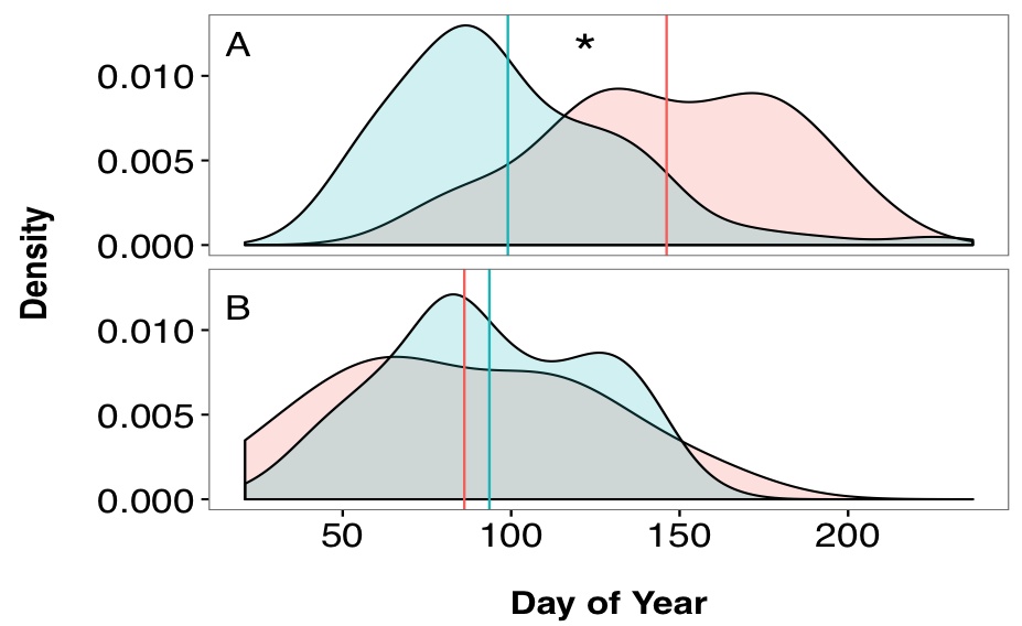
Figure 4.1: Comparisons of hatch date distributions (estimated from otolith-based reconstructions) for sampled adults (pink) and juveniles (blue) of G. maculatus. Panel (A): Hutt River. Panel (B): Wainuiomata River. Vertical line indicates mean hatch date for each group. Asterisk indicates dissimilar distributions and mean values based on the Anderson-Darling test and one-way ANOVA.

4.3.2 Shifts in juvenile growth histories

Growth histories of fish sampled from the Hutt River differed significantly among sampled dates (i.e., among cohorts and/or between juvenile and adult age classes; F4, 339 = 13.091, p < 0.0001), indicating that different groups of fish had different otolith growth curves. The parameter estimates of the model showed that the otolith growth histories of fish caught in August, September and October all had significantly faster otolith growth rates relative to the adult fish (Aug: T339 = 5.1774, p < 0.0001; Sep: T339 = 4.7295, p < 0.0001; Nov: T339 = 2.2944, p = 0.0224, 4.2A). Fish caught in November did not show a significantly different otolith growth curve to the adult fish (T339 = 0.2103, p = 0.8336, 4.2A).

Growth histories of fish sampled from the Wainuiomata River also varied significantly among sampled dates (F3, 198 = 5.636, p = 0.001). Parameter estimates of the model showed that the otolith growth histories of fish from August and September were significantly different to the adult fish (Aug: T198 = 2.3467, p = 0.0199; Sep: T198 = 2.2317, p = 0.0268, 4.2B). Fish caught in October did not show significantly different otolith growth histories to the adult fish (T198 = 0.1748, p = 0.8614, 4.2B).

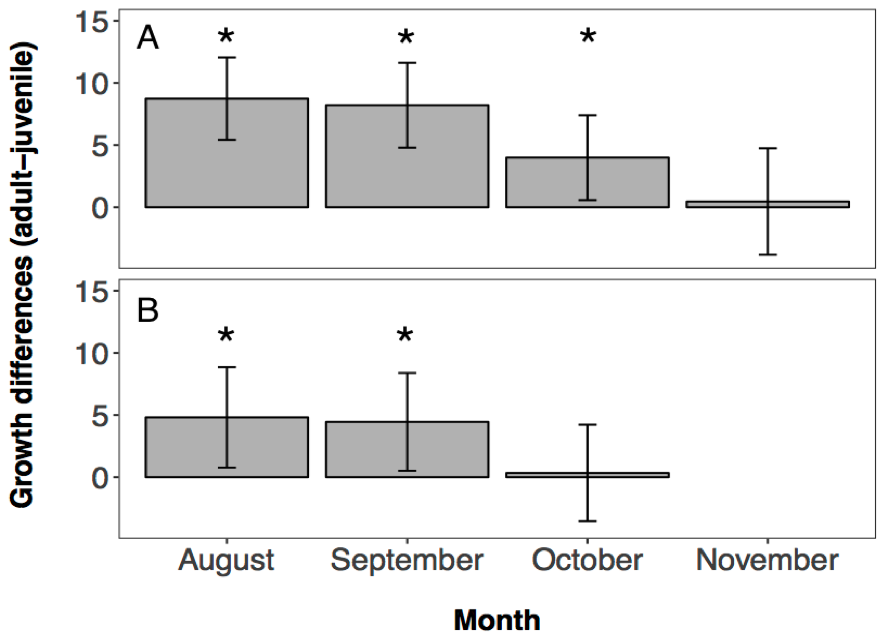
Figure 4.2: Estimates of otolith growth for each juvenile cohort from (A) the Hutt River, and (B) the Wainuiomata River ±95% CI. Model calculates juvenile growth estimates relative to the adult growth estimates. Therefore any estimate that is approximately zero represents a juvenile otolith growth that is equal to the adult otolith growth. Values above zero reflect faster juvenile growth compared to adult survivor growth. Asterisks represent otolith growth estimates significantly different from zero. No fishing was conducted in the Wainuiomata River in November due to river mouth closure.

4.4 Discussion

The main purpose of this chapter was to understand how hatch date and growth history collectively shape survival in post-settlement fish. Similarly to results from Chapter 2, each site exhibited different patterns. In the Hutt River, hatch date distributions differed strongly between adult fish and juvenile fish. However, in the Wainuiomata River, there was no difference in hatch date distribution between life stages. Adult populations from both rivers had relatively slow growth compared to the juvenile fish. This slower growth also correlated with the growth rate of juvenile fish entering the river in November (in the Hutt River) and October (in the Wainuiomata River).

Shifts in hatch date distributions differed between each site. The interpretation of this result is constrained by the mismatch in sampling of adult G. maculatus between the two study sites, and the overall limited sampling of adult fish. However, if the samples are an accurate reflection of hatch date distributions, then the spatial differences observed here could potentially be attributed either to different post-settlement processes operating in each river, or it may be a function of different phenotypic mixtures of juvenile fish entering each river. Chapters 2 and 3 indicated that there were considerable differences in the phenotypes of juvenile fish between each site. Therefore, the input of phenotypically distinct cohorts into each river may be responsible for the observed difference in adult composition. Fish entering the Wainuiomata River were more phenotypically homogenous, whereas fish entering the Hutt River were more phenotypically heterogeneous (based on Chapter 2 results). If the Hutt River has a more phenotypically diverse population of G. maculatus, then fitness linked traits like hatch date and growth rate may have larger population level effects, relative to a more homogenous population (McCauley et al. 1993). Juvenile fish entering the Hutt River may have spent time in different environments and/or were from different natal sources. This environmental heterogeneity may drive differences in growth rate, which in turn affected their freshwater survival (Shima and Swearer 2010). Therefore, post-settlement processes in each river may actually be identical, but they produce different results in each river as they are acting on the phenotypes of the G. maculatus population. This may have interesting implications for my results from Chapter 3, as there I suggested that mortality patterns were indiscriminate to phenotype. Correlations between fitness and phenotypic traits may vary depending on G. maculatus life stage, and therefore early life experiences may have considerable flow on effects to later life stages (Meekan et al. 2010)

Fish from both rivers showed similar (but not identical) shifts in growth rate distributions. My results suggest that adult fish had comparatively slow otolith growth rates in their early life history. Again, interpretation of these results is constrained by the limited adult sampling. Shifts in the phenotypic distributions between juveniles and adults may simply be the result of sample bias. However, if they are an accurate reflection of traits at each life stage, then there are several possibilities for these patterns. In many systems, growth rate may be linked to fitness, and fish often experience selective mortality on life history traits after settlement (Vigliola and Meekan 2002, Raventós and Macpherson 2005, Vigliola et al. 2007, Shima and Swearer 2010). Predation has been shown to be an important source of post-settlement mortality in other systems (Shulman 1985, Hixon 1991, Connell 1996, Webster 2002), and is known to be a strong factor in structuring freshwater fish communities (Goodgame and Miranda 1993, Kohler et al. 1993, Jackson et al. 2001, Santucci Jr and Wahl 2003), particularly when the predators are introduced species (Li and Moyle 1981). G. maculatus are preyed on by introduced trout (Crowl et al. 1992, Glova 2003, Bonnett and McIntosh 2004, Vigliano et al. 2009), and this predation may be selective towards certain life history traits (Werner and Hall 1974, Hambright 1991, Green and Côté 2014). Therefore, a potential explanation for the shift in adult phenotypes towards slower growth rates may be that selective mortality is operating on post-settlement G. maculatus.

Adult fish in the Hutt River had significantly different hatch dates to the juvenile fish hatch dates. A considerable body of literature has indicated that hatch date can influence survival, with evidence that either early (Confer and Cooley 1977, Houde 1989, Schupp 1990, Cargnelli and Gross 1996), or late hatching (Garvey et al. 2002, Santucci Jr and Wahl 2003, Kaemingk et al. 2013) can benefit survival. However, my results indicate that an early vs late dichotomy may not be representative for this species. Instead, fitness may be dependent upon hatching at an ‘optimal’ time that maximizes exposure to the best environmental conditions, affording suitable growth rates for the next life stage and environments. Hatching at the ‘wrong’ time may result in larvae having lower food availability (Cargnelli and Gross 1996), or experiencing less favourable environmental conditions (Kramer and Smith Jr 1962, Mooij et al. 1994). These conditions may influence phenotypic variation (i.e. alter growth rates), which may set them up better for future success (Shima and Swearer 2010). Therefore, hatch date may not directly influence freshwater survival, but it could expose fish to a range of time- (or seasonally-) dependent conditions during their marine dispersal phase.

While there is evidence that slow growth can be detrimental to young fish (Crecco and Savoy 1985, Post and Prankevicius 1987, Danylchuk and Tonn 2001, Vigliola et al. 2007), most of the support for the ‘bigger-is-better’ hypothesis comes from systems where predators become gape-limited (Perez and Munch 2010). In systems where prey never outgrow the gape of predators, fast growth may prove to be detrimental (Litvak and Leggett 1992, Bertram and Leggett 1994). Larger fish are more likely to be encountered, and attacked by predators (Fuiman 1989, Litvak and Leggett 1992), whereas smaller fish can be more inconspicuous. Larger fish are also known to feed in food rich microhabitats, which often increases susceptibility and vulnerability to predators (Biro et al. 2006). Cushing (1990) suggested that the best survival came from fish that could spend the least amount of time at a vulnerable size (i.e., the stage-duration hypothesis). However, it is unlikely that G. maculatus ever reach a size where they are not vulnerable to predation (Glova 2003), and therefore, remaining small and inconspicuous may offer them the best chances for survival.

All fish that were older than 180 days had their growth profiles truncated so that 180 was the maximum age observed. Otolith growth can decouple from somatic growth post settlement (Hoey and McCormick 2004) and I did not want this post-settlement growth to be considered by the mixed effects model. 180 days was chosen as it was the approximate age of the average juvenile fish, and therefore I considered it a good approximation of the adult fish age at settlement. However, this approach makes the assumption that the adult fish are part of the same cohort as the juvenile fish, and indeed that using an ‘average age’ is a good way to estimate their pre-settlement growth. The missing link to this puzzle lies in the adult fish age-at-settlement. A ‘settlement mark’ has been validated for G. maculatus (Hale and Swearer 2008), however I was unable to locate a settlement mark in any of the adult otoliths, and thus I was unable to estimate age-at-settlement. In reality, adult survivors may be settling at a very different age to the recruiting juvenile fish population and this ‘age effect’ may be the factor driving survivorship for certain individuals. As this data simply isn’t known, I believe that using an ‘average age’ is an acceptable method for analysis of growth histories. Future studies could use more sophisticated techniques (i.e. LA-ICPMS, as per Hale and Swearer 2008) to consistently identify this settlement mark and confirm whether adult fish are settling at similar ages.

Although the evidence presented in this chapter is circumstantial, it has generated a novel hypothesis for the role of growth rate on individual success in G. maculatus. Growth rate appears to be important in freshwater populations of G. maculatus, however, results from Chapter 3 indicated that growth may not be tightly linked with fitness in marine populations. This has implications for our understanding of the ecology of G. maculatus, and suggests that fitness linked traits may change with ontogeny. Hatch date may also have strong influences, as larval rearing environment will likely shape juvenile growth rates. Future directions should use experimental approaches to investigate predator-induced selective mortality on G. maculatus (i.e. through mesocosm approaches, Parker 1971), and unravel the role of growth rate in both marine and freshwater populations.