3 Implications of Variable Larval Quality on Juvenile Mortality in Galaxias Maculatus
3.1 Introduction
Marine organisms with stage structured life histories can experience very high mortality rates during their planktonic phase (Hjort 1914, Bailey and Houde 1989). This level of mortality can be mediated by growth rates, where selective mortality favours individuals with specific patterns of growth (Anderson 1988). Fast growth may be beneficial if it enables fish to outgrow gape limitations of predators (Hambright 1991), improve upon their swimming ability to escape predators (Litvak and Leggett 1992), and/or store sufficient energy to avoid starvation (Shuter et al. 1980, Conover and Schultz 1997). Conversely, slow growth can be beneficial if fish become more inconspicuous to predators (Biro et al. 2004) or undertake behavioural changes to minimise their vulnerability (Meekan et al. 2010)
An individual’s growth rate may be correlated with its rearing environment. Biotic and abiotic factors may influence the magnitude of growth rate, resulting in phenotypes being partially influenced by developmental environment (Agrawal 2001). Environmental variables known to influence growth rate include temperature (Green and Fisher 2004), presence of predators (Milano et al. 2006), water movement (Kekalainen et al. 2010), and food availability (Jones 1986), although relationships may be positive, negative, and/or non-linear. Optimal temperatures and food availability will usually promote higher levels of growth (MacDonald and Thompson 1985) although these relationships can be complex and context dependent (Nicieza and Metcalfe 1997). A substantial body of evidence indicates that growth is also linked with fitness (Cowan et al. 1996, Searcy and Sponaugle 2001, Shima and Findlay 2002, Raventós and Macpherson 2005, Grorud-Colvert and Sponaugle 2006, Shima and Swearer 2009), with further evidence indicating that increases in fitness may be linked with growth in early life (Shima and Findlay 2002, Gagliano et al. 2007), and growth immediately preceding life stage transitions (Hamilton 2008, Hamilton et al. 2008). In species with protracted spawning and a pelagic dispersal phase, separate cohorts of fish may experience different conditions due to natural temporal variation in the environment (i.e. across seasons). Long distance dispersal can be a physiologically demanding event, and often results in high levels of mortality (Baker and Rao 2004).
There are well defined conceptual frameworks for the relationship between growth and mortality (Anderson 1988). The growth-mortality hypothesis (Ware 1975, Shepherd and Cushing 1980) generally predicts that growth will be related to mortality, typically through the mechanisms of starvation and/or predation. However, both of these processes typically elucidate different relationships between growth and mortality (Anderson 1988, Leggett and Deblois 1994). Limitation by food can lead to a relationship where fish with higher growth rates experience lower mortality. Prey can often be distributed non-uniformly, and it has been suggested that ambient prey density in the ocean is too low to support growth and survival of larval fish (Anderson 1988). Larger larvae are less susceptible to starvation than smaller conspecifics, due to having excess fat reserves (Hjort 1914), and therefore are more likely to survive intense periods of starvation (i.e., over winter mortality). Growth and mortality would therefore show an inverse relationship, where fish with higher growth rates would experience lower levels of mortality.
Limitation by predators can show a different relationship, where prey mortality follows a dome shaped curve. Under this model, fish with the highest and lowest growth rates will experience the highest levels of mortality. Fish are the most significant predators of fish larvae (Pepin 1987, Bailey and Houde 1989) and they are known to cause significant levels of mortality (Ware 1975, Sissenwine 1984, Gaines and Roughgarden 1987, Bailey and Houde 1989). Predation by fish requires larvae to be encountered, attacked, and captured (Pepin 1992). Small fish with have a low encounter rate, but a high capture rate, whereas large fish will have a high encounter rate with a low capture rate, thus producing the relationship where intermediate sizes convey the highest fitness (Leggett and Deblois 1994).
Here, I examine how mortality varies as a function of larval quality in an amphidromous fish (Galaxias maculatus) during a migratory phase in its life cycle. Adult G. maculatus are primarily semelparous (McDowall 1968, but see Stevens et al 2016). Across a population, however, spawning occurs over a period of several months. Larvae spend 3-6 months developing in the open ocean before migrating (as metamorphosed juveniles) to freshwater streams, where they develop for a further ~six months before spawning (McDowall 1990). In New Zealand, upstream migration occurs year round, however migration peaks from August to November (McDowall et al. 1994). Environmental conditions (e.g. temperature, food availability) vary over the recruitment period, setting up an expectation for temporal variation in the quality of incoming recruits. I build on my results from chapter 2 by exploring the relationship between phenotypic ‘quality’ and mortality rates. Specifically, I used the same samples of fish from the methodology in chapter 2 and used otolith based reconstructions of fish life histories to derive a measure of larval quality. I quantified the mortality rates experienced by each daily cohort, and investigated whether these two traits were interrelated. As larval fish are susceptible to both starvation and predators, I hypothesised that the relationship between mortality and larval quality would follow either the linear, food-limited trend, or the dome-shaped, predation-limited trend.
3.2 Methods
3.2.1 Fish collections
Briefly, I sampled incoming G. maculatus recruits from two rivers in the Wellington area. Sampling was conducted so that fish were collected across the main recruitment season (August to November). For a full description of juvenile sampling, see chapter 2.
3.2.2 Characterising larval quality
Following the general approach of Shima and Swearer (2009), I used the daily otolith increments to estimate four variables that describe the phenotypic ‘quality’ of incoming G. maculatus recruits: (1) “Pelagic larval duration” (PLD) is an estimate of the time the individual has spent developing as a larvae, and was estimated as the number of daily rings. (2) “Average growth rate” is a measure of the average amount of somatic growth an individual experienced on a given day, and was estimated as the average distance between successive daily rings. (3) “Early growth rate” was estimated as the average distance between the first 20 daily rings. (4) “Late growth rate” was estimated as the average distance between the last 20 daily rings.
I centered and scaled the four variables (mean = 0, SD = 1) and performed a principal components analysis, using the ‘prcomp’ function in RStudio v0.99.903 (RStudio Team 2015) , to derive a composite metric of ‘larval quality’ score (i.e., first principal component).
3.2.3 Estimating mortality rates
To estimate mortality rates I used the Chapman-Robson approach to catch-curve analysis (Chapman and Robson 1960, Robson and Chapman 1961). Catch curve analysis is used to estimate mortality by measuring the decline of the number of individuals in the age classes of a cohort (Pauly 1990). Traditional catch-curve analysis (Ricker 1975) would fit a linear regression to the descending limb of an age-frequency curve, under the assumption that the ascending limb of the curve contains fish too young to recruit to the fishery or gear. The Chapman-Robson method instead treats the descending limb of the curve as following a geometric probability distribution, and computes a maximum likelihood estimator for annual survival (Chapman and Robson 1960, Robson and Chapman 1961). Instantaneous mortality rates (Z) can then be computed using Z=-log(annual mortality), however these estimates have be shown to be slightly biased, so I instead used the correction offered by Hoeing et al (1983). The Chapman-Robson approach was chosen over more traditional methods due to the findings of Dunn et al (2002) and Smith et al (2012) who showed that this method is the most precise, and produces the least variance. All calculation of Z scores was done with the ‘FSA’ package (Ogle 2016) in RStudio v0.99.903 (RStudio Team 2015).
3.2.4 Evaluating the relationship between mortality and quality
For this analysis, I assumed that samples collected on different days were independent of one another (i.e. I did not model the temporal structure of my sampling design; c.f. Chapter 2). For each sample day at each site I computed average larval quality and instantaneous mortality rate (i.e., estimated for fish collected from a given site on the same day). Because preliminary analysis (loess regression) indicated a linear relationship between instantaneous mortality and larval quality, I used a linear model for my formal analysis. Specifically, I used an ANCOVA model to evaluate the relationship between instantaneous mortality (the response variable) and larval quality (the covariate), and whether the intercept and/or the slope of this relationship varied between sites.
3.3 Results
The first principal component accounted for 54% of the variation in the larval quality variables. PLD loaded positively on PC1, while the three growth variables all loaded negatively. Fish with higher PC1 scores therefore had long PLDs with slow growth. Since a low PC1 score would indicate a fish of higher ‘quality’ (i.e., faster growth and development time), I multiplied all PC1 scores by -1 for purposes of presentation (i.e. so that the re-expressed PC1 scores scale more intuitively with traits often associated with ‘larval quality’.
3.3.1 Relationship between mortality and larval quality
The relationship between instantaneous mortality rate and average larval quality was consistent across sites (interaction term: F1,17 = 1.3262, p = 0.2654). Therefore I evaluated a reduced model using only main effects of larval quality and site. Instantaneous mortality rates did differ between sites (F1,18¬ = 0.0891, p = 0.7688), and there was no significant relationship between instantaneous mortality rates and larval quality (F1,18 = 3.2712, p = 0.0872). Although the model was not significant, there does appear to be a trend towards higher quality fish experiencing lower mortality (3.1). The power of the model was very low (0.2751) based off detecting a ‘medium’ effect size, so non-significance may be attributable to insufficient sample size. Power analysis indicated that a sample of ~60 would give the model a more reasonable power of 0.8.
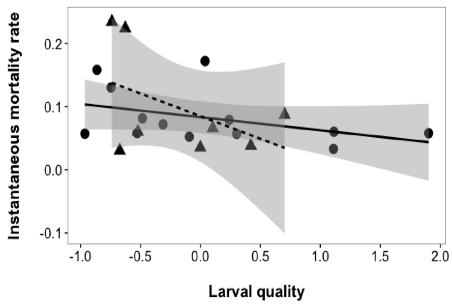
Figure 3.1: Relationship between instantaneous mortality rate (Z score) and average larval quality (PC1) for each daily cohort of G. maculatus from two sites: circle/solid line = Hutt River, triangle/dashed line = Wainuiomata River. Shaded lines represent the 95% confidence interval around the regression lines.
3.4 Discussion
Few studies have addressed threats during the marine phase of the G. maculatus life cycle (Barriga et al. 2007, Jellyman and McIntosh 2008). Fish undertaking dispersal in the open ocean can be subject to environmental factors, such as temperature (Pepin 1991) and food (Einum 2003) fluctuations, that may cause changes in growth rate. Understanding changes in growth, and how it relates to mortality rates, may provide information on factors that constrain fish populations during dispersal. Growth-mortality relationships are often non-linear (e.g. U-shaped), where highest mortality is experienced by the fastest and slowest growers (Anderson 1988, Staudinger and Juanes 2010), or negatively linear, where highest mortality is experienced by the slowest growers (Leggett and Deblois 1994). However, my results did not appear to follow either of these trends.
Phenotype is at least partially influenced by environment (Meekan et al. 2003, Sponaugle et al. 2006), and cohorts of G. maculatus with varying dispersal pathways may show evidence of this through their phenotype. My previous chapter demonstrated site specific differences in growth rates, yet here site was unrelated to differences in mortality rates. These results suggest that mortality is not a function of dispersal pathway (assuming different phenotypes from Chapter 2 would result in different mortality rates), and is experienced consistently across spatial scales. While environmental variation may be strong enough to significantly differentiate phenotypes between spatially separated cohorts, it may not cause differing levels of mortality in larval G. maculatus. While G. maculatus are known to have high levels of phenotypic plasticity (Barriga et al. 2002), it appears that factors governing mortality are either unrelated to phenotype, or they are shared, both in direction and magnitude, producing similar larval quality distributions.
Instantaneous mortality rate also appeared to be unrelated with larval quality. My results did show a weak negative trend, which would be a characteristic of food limitation, however this trend was non-significant. The model used to evaluate this relationship had very low power (0.2751), which may have constrained its ability to detect a significant relationship, however my results seem to suggest that a factor other than food or predators is causing mortality in cohorts of G. maculatus. While starvation and predation are some of the strongest forces affecting larval survival (Leggett and Deblois 1994), it is important to consider that there are multiple sources of mortality that affect larvae (Pineda et al. 2009). Specifically, catch-curve analyses do not consider mortality due to advection, and transport away from suitable settlement habitat (White et al. 2014). Therefore, an alternative interpretation is that my mortality estimates have assumed the mortality of recruits that are still alive, but were transported away from my study areas and settled elsewhere. Thus, they are presumed dead by the catch-curve model (due to not being sampled). Therefore, while the study of larval transport and retention is important in understanding phenotypic patterns (c.f. Chapter 2), it may also be important in understanding mortality patterns.
An alternative explanation for my results is that my sampling may reflect a population that has already experienced extensive selective mortality. Sampled fish may only represent the survivors, and therefore my sampling may have not captured the ‘larval quality’ scores of fish that experienced strong mortality pressures. Therefore, the relationship between quality and mortality may have originally followed a more typical U-shaped relationship (Anderson 1988) but, post-mortality, only the centre of this spectrum remains (or some segment of this pattern). As the more extreme edges of the growth-mortality curve may not be able to be detected, the non-linear relationship becomes masked to this analysis. Overcoming this limitation in future studies may be difficult, and require extensive sampling of larval G. maculatus during their marine dispersal phase.
This lack of mortality due to abiotic factors ties in further with my results from Chapter 2. While not explicitly evaluated in this chapter, fish from the Hutt River appears to have a wider range of larval quality scores, but a smaller range of mortality rates, than fish from the Wainuiomata River (3.1). These are similar results to Chapter 2, where I found strong spatial differences in phenotypes between each river. Similarly to Chapter 2, this result could indicate a more heterogeneous rearing environment (i.e., environmental experience hypothesis), which allows a greater scope for extreme phenotypes to persist. Wellington Harbour may act as a ‘nursery’ ground, where environmental heterogeneity drives phenotypic differentiation, but also provides more refuge from lethal effects (i.e., as seen in the lower variability in mortality rate, 3.1).
Estimates of instantaneous mortality rates based upon catch-curve analyses depend upon several important assumptions (Ricker 1975). Specifically, it assumes that the population being tested is closed, with no immigration or emigration, and that all age classes are equally recruited to the fishing gear. Populations of G. maculatus are generally considered to be demographically open (Waters et al. 2000), due to their significant dispersal capabilities, however, other studies have used this technique on open populations (Sandström and Thoresson 1988, Irvine et al. 2007, Windsland 2014). The assumption of a closed population is assuming a study system with a standing stock of individuals, of which recruits are added to through time (Ricker 1975). G. maculatus typically die at one year of age, and so my sampling does not reflect mortality in a standing stock, rather, it is only considering these new recruits. In essence, this analysis is based around a daily stock recruitment model, rather than an annual one. Furthermore, Ricker’s initial methodology was based around using fish that were grouped into year classes rather than day classes, and most subsequent applications of the method have used year class fish (Hoffnagle and Timmons 1989, Restrepo et al. 2007, Kell et al. 2013). However, the technique has been applied to day class fish (Essig and Cole 1986) and to G. maculatus specifically (Barriga et al. 2012). Due to the prevalence of this technique, and that I am only treating each daily cohort as a closed population, I believe that my results are robust enough to be interpreted with caution. While I do not claim they represent a ‘true’ measure of mortality, they are still useful to draw inference from.
This study has demonstrated that there appears to be little relationship with the quality of recruiting G. maculatus and their relative mortality rates. There did appear to be a trend towards lower rates of mortality when fish were higher quality, but this may require higher sample sizes and longitudinal sampling of a cohort to validate. These results suggest that understanding dispersal may be a critical factor in studies of mortality, and that sources of mortality may operate indiscriminately on phenotypically different populations. They also suggest that a ‘phenotypically’ superior G. maculatus individual may not experience lower mortality, and have therefore have implications for the carry-over effects that individuals may experience post-settlement.